Sorting Algorithms

Sorting is a process of arranging elements in increasing or decreasing order. There are different ways of classifying the algorithms, like time complexity, space complexity, stability, Internal/external sorting, recursive/non-recursive sortings.

The major Sorting techniques are

1)-Insertion Sort O(N²) 

2)-Bubble Sort O(N²) 

2)-Selection sort O(N²) 

3)-Quick Sort O(N²)

4)-Merge Sort O(NlogN)

5)-Heap Sort O(NlogN)

6)-Bucket Sort (depends on algo. of bucket)

7)-Counting Sort (O(n+k) )

8)-Radix Sort O(d*(n+b)) 

Lets discuss one by one in detail.

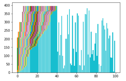
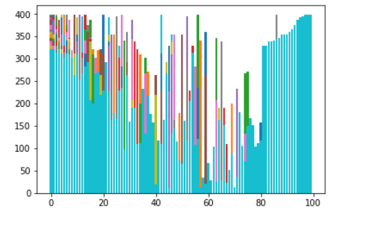
Insertion Sort

Insertion Sort is a simple comparison based sorting algorithm. It inserts every array element into its proper position. In i-th iteration, previous (i-1) elements (i.e. subarray Arr[1:(i-1)]) are already sorted, and the i-th element (Arr[i]) is inserted into its proper place in the previously sorted subarray

Time Complexity:

• Best Case Sorted array as input, [ O(N) ]. And O(1) swaps.
• Worst Case: Reversely sorted, and when inner loop makes maximum comparison, [ O(N²) ] . And O(N²) swaps.
• Average Case: [ O(N²) ] . And O(N²) swaps.

Space Complexity: [ auxiliary, O(1) ]. In-Place sort.

Advantage:

1. It can be easily computed.
2. Best case complexity is of O(N) while the array is already sorted.
3. Number of swaps reduced than bubble sort.
4. For smaller values of N, insertion sort performs efficiently like other quadratic sorting algorithms.
5. Stable sort.
6. Adaptive: total number of steps is reduced for partially sorted array.
7. In-Place sort.

Disadvantage:

1. It is generally used when the value of N is small. For larger values of N, it is inefficient.

Code:

def insertion(data):

    selection=1

    data_range=len(data)

    while selection<data_range:

        for i in range(selection):

            if(data[selection]<data[i]):

                temp=data[i]

                data[i]=data[selection]

                data[selection]=temp

        selection+=1

        showGraph()

    return data

end=time.time()

Uses: Insertion sort is used when number of elements is small. It can also be useful when input array is almost sorted, only few elements are misplaced in complete big array.

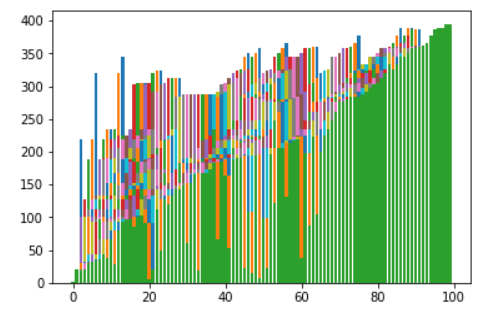
Bubble Sort

Bubble Sort is repeatedly compares and swaps(if needed) adjacent elements in every pass. In i-th passof Bubble Sort (ascending order), last (i-1) elements are already sorted, and i-th largest element is placed at (N-i)-th position, i.e. i-th last position.

Time Complexity:

• Best Case Sorted array as input. Or almost all elements are in proper place. [ O(N) ]. O(1) swaps.
• Worst Case: Reversely sorted / Very few elements are in proper place. [ O(N²) ] . O(N²) swaps.
• Average Case: [ O(N²) ] . O(N²) swaps.

Space Complexity: A temporary variable is used in swapping [ auxiliary, O(1) ]. Hence it is In-Place sort.

Advantage:

1. It is the simplest sorting approach.
2. Best case complexity is of O(N) [for optimized approach] while the array is sorted.
3. Using optimized approach, it can detect already sorted array in first pass with time complexity of O(1).
4. Stable sort: does not change the relative order of elements with equal keys.
5. In-Place sort.

Disadvantage:

1. Bubble sort is comparatively slower algorithm.

Code

def bubbleSort():

    n = len(data)

    maximum=len(data)

    # Traverse through all array elements

    for i in range(n):

        # Last i elements are already in place

        for i in range(maximum-1,1,-1):

            for j in range(0,i):

                if (data[j]>data[j+1]):

                    temp=data[j+1]

                    data[j+1]=data[j]

                    data[j]=temp

            showGraph()

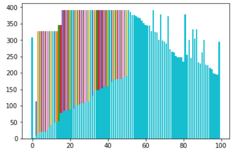
Selection Sort

The selection sort algorithm sorts an array by repeatedly finding the minimum element (considering ascending order) from unsorted part and putting it at the beginning. The algorithm maintains two subarrays in a given array.

1) The subarray which is already sorted.
2) Remaining subarray which is unsorted.

Time Complexity:

• Best Case [ O(N²) ]. Also O(N) swaps.
• Worst Case: Reversely sorted, and when inner loop makes maximum comparison. [ O(N²) ] . Also O(N) swaps.
• Average Case: [ O(N²) ] . Also O(N) swaps.

Space Complexity: [ auxiliary, O(1) ]. In-Place sort.

Advantage:

1. It can also be used on list structures that make add and remove efficient, such as a linked list. Just remove the smallest element of unsorted part and end at the end of sorted part.
2. Best case complexity is of O(N) while the array is already sorted.
3. Number of swaps reduced. O(N) swaps in all cases.
4. In-Place sort.

Disadvantage:

1. Time complexity in all cases is O(N²), no best case scenario

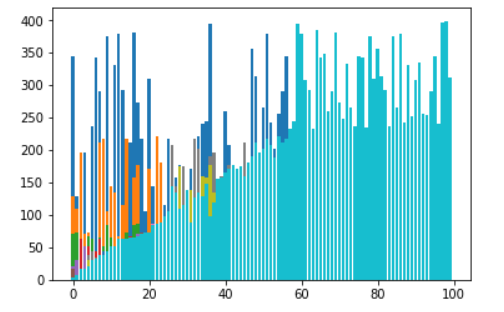
Quick Sort

QuickSort is a Divide and Conquer algorithm. It picks an element as pivot and partitions the given array around the picked pivot. There are many different versions of quickSort that pick pivot in different ways.

1. Always pick first element as pivot.
2. Always pick last element as pivot (implemented below)
3. Pick a random element as pivot.
4. Pick median as pivot.

The key process in quickSort is partition(). Target of partitions is, given an array and an element x of array as pivot, put x at its correct position in sorted array and put all smaller elements (smaller than x) before x, and put all greater elements (greater than x) after x. All this should be done in linear time.

There are certain reasons due to which quicksort is better especially in case of arrays:

1. Auxiliary Space : Mergesort uses extra space, quicksort requires little space and exhibits good cache locality. Quick sort is an in-place sorting algorithm. In-place sorting means no additional storage space is needed to perform sorting. Merge sort requires a temporary array to merge the sorted arrays and hence it is not in-place giving Quick sort the advantage of space.
2. Worst Cases : The worst case of quicksort O(n²) can be avoided by using randomized quicksort. It can be easily avoided with high probability by choosing the right pivot. Obtaining an average case behavior by choosing right pivot element makes it improvise the performance and becoming as efficient as Merge sort.
3. Locality of reference : Quicksort in particular exhibits good cache locality and this makes it faster than merge sort in many cases like in virtual memory environment.
4. Merge sort is better for large data structures: Mergesort is a stable sort, unlike quicksort and heapsort, and can be easily adapted to operate on linked lists and very large lists stored on slow-to-access media such as disk storage or network attached storage.
5. following.

Merge Sort

Merge Sort is a Divide and Conquer algorithm. It divides input array in two halves, calls itself for the two halves and then merges the two sorted halves. The merge() function is used for merging two halves. The merge(arr, l, m, r) is key process that assumes that arr[l..m] and arr[m+1..r] are sorted and merges the two sorted sub-arrays into one. 

In case of linked lists the case is different mainly due to difference in memory allocation of arrays and linked lists. Unlike arrays, linked list nodes may not be adjacent in memory. Unlike array, in linked list, we can insert items in the middle in O(1) extra space and O(1) time. Therefore merge operation of merge sort can be implemented without extra space for linked lists.

Time Complexity

The time complexity of MergeSort is same in all 3 cases (worst, average and best) as merge sort always divides the array into two halves and take linear time to merge two halves.

Auxiliary Space: O(n)

Algorithmic Paradigm: Divide and Conquer

Heap Sort

Heap sort is a comparison based sorting technique based on Binary Heap data structure. It is similar to selection sort where we first find the maximum element and place the maximum element at the end. We repeat the same process for remaining element.

Its typical implementation is not stable, but can be made stable 

Time Complexity: Time complexity of heapify is O(Logn). Time complexity of createAndBuildHeap() is O(n) and overall time complexity of Heap Sort is O(nLogn).

Heap Data Structure is generally taught with Heapsort. Heapsort algorithm has limited uses because Quicksort is better in practice. Nevertheless, the Heap data structure itself is enormously used. Following are some uses other than Heapsort.

Priority Queues: Priority queues can be efficiently implemented using Binary Heap because it supports insert(), delete() and extractmax(), decreaseKey() operations in O(logn) time. Binomoial Heap and Fibonacci Heap are variations of Binary Heap. These variations perform union also in O(logn) time which is a O(n) operation in Binary Heap. Heap Implemented priority queues are used in Graph algorithms like Prim’s Algorithm and Dijkstra’s algorithm.

Code

def heapSort(arr): 

    n = len(arr) 

    # Build a maxheap. 

    for i in range(n, -1, -1): 

        heapify(arr, n, i) 

        showGraph()

    # One by one extract elements 

    for i in range(n-1, 0, -1): 

        arr[i], arr[0] = arr[0], arr[i]   # swap 

        heapify(arr, i, 0)

        showGraph()

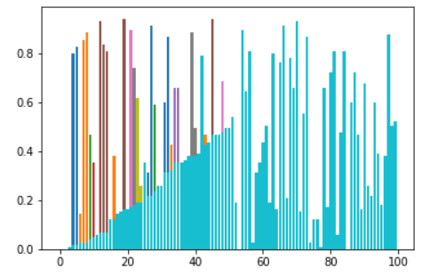
Bucket Sort

Bucket sort is mainly useful when input is uniformly distributed over a range. For example, consider the following problem. 
Sort a large set of floating point numbers which are in range from 0.0 to 1.0 and are uniformly distributed across the range.

The overall performance would then be dominated by the algorithm used to sort each bucket, which is typically O(n^2) Insertion sort, making bucket sort less optimal than O(n log n) Comparison sort algorithms like Quick sort.

def bucketSort(x): 

    arr = []

    slot_num = 100

    # 10 means 10 slots, each 

    # slot's size is 0.1

    for i in range(slot_num): 

        arr.append([])

        # Put array elements in different buckets

    for j in x:

        index_b = int(slot_num*j)

        #print(index_b)

        arr[index_b].append(j)

    # Sort individual buckets  

    for i in range(slot_num): 

        arr[i] = insertionSort(arr[i])

    # concatenate the result

    k = 0

    for i in range(slot_num):

        for j in range(len(arr[i])):

            x[k] = arr[i][j]

            k += 1

        showGraph()

    return x

Counting Sort

Counting sort is a sorting technique based on keys between a specific range. It works by counting the number of objects having distinct key values (kind of hashing). Then doing some arithmetic to calculate the position of each object in the output sequence.

Time Complexity: O(n+k) where n is the number of elements in input array and k is the range of input.
Auxiliary Space: O(n+k)

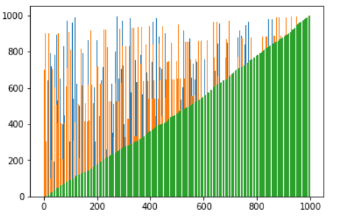
Radix Sort

The lower bound for Comparison based sorting algorithm (Merge Sort, Heap Sort, Quick-Sort .. etc) is Ω(nLogn), i.e., they cannot do better than nLogn.

Counting sort is a linear time sorting algorithm that sort in O(n+k) time when elements are in range from 1 to k.

What if the elements are in the range from 1 to n²? 
We can’t use counting sort because counting sort will take O(n²) which is worse than a comparison based sorting algorithms. Can we sort such an array in linear time?
Radix Sort is the answer. The idea of Radix Sort is to do digit by digit sort starting from least significant digit to most significant digit. Radix sort uses counting sort as a subroutine to sort.

Time Complexity

Let there be d digits in input integers. Radix Sort takes O(d*(n+b)) time where b is the base for representing numbers, for example, for decimal system, b is 10. What is the value of d? If k is the maximum possible value, then d would be O(log_b(k)). So overall time complexity is O((n+b) * log_b(k)). 

Code

def radixSort(arr): 

    # Find the maximum number to know number of digits 

    max1 = max(arr) 

    # Do counting sort for every digit. Note that instead 

    # of passing digit number, exp is passed. exp is 10^i 

    # where i is current digit number 

    exp = 1

    while max1/exp > 0: 

        countingSort(arr,exp)

        exp *= 10

        showGraph()

References:
https://www.geeksforgeeks.org/quick-sort-vs-merge-sort/

Note: Please write to us at machine.intellegence@gmail.com to report any issue with the above content. The above content is just as reference material. We are not claiming it as intellectual property.