Algebra

Today, I am going to tell you a story of a Philosopher, Mr.Mathematics. He is a philosopher of calculation. He is as old as the sun or the moon. With his philosophy, we measure distance, predict the basics of time. His wife is Lady Calculation. She is intellectual, smart and honest. Now I know you want to know their sons. They have two sons, Arithmetic and Algebra.

The Family of Philosopher

Arithmetic knows what is known and solves the philosophy of addition, subtraction, Multiplication, and Division. So we may say that he can solve 5+6=?.

Algebra the younger sons with the power of his mother he replaces the known by alphabets. So we may say that he can solve x+y=?.

I know you all are looking on who is that young girl, she is Matrix. The Daughter of Algebra. Actually, Algebra has one Daughter and three sons Vector, Scalar and Tensor.

Vector: He is expert in managing the things with magnitude and direction.

Scalar: He is like the vector but inefficient in managing the things in a direction.

Tensor: He is having the power of vector and matrix.

Algebra has one more power, he can help in visualizing the things by using its Linear or Quadratic equations.

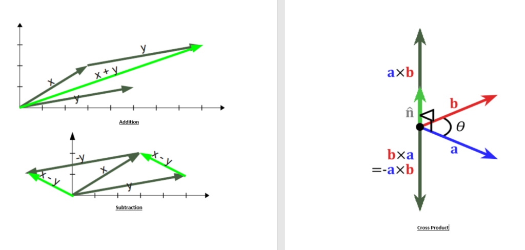
So let us start with some coding. We have two matrices as shown in below code we try to add both the matrix.

#A matrix Addition

from mpl_toolkits.mplot3d import Axes3D
import numpy as np
import matplotlib.pyplot as plt

fig = plt.figure()
ax = fig.gca(projection='3d')

# Plot the first line
x1 = [0,6]
y1 = [0,12]
ax.plot(x1, y1, zs=0, zdir='z', label='curve in (x,y)')

# Plot the second line
x2 = [0,0]
y2 = [0,14]
ax.plot(x2, y2, zs=0, zdir='z', label='curve in (x,y)')

#plot the third line
x3 = np.array(x1)+np.array(x2)
y3 = np.array(y1)+np.array(y2)


ax.plot(x3,y3, zs=0, zdir='z', label='curve in (x,y)')

plt.show()

OutPut: The Green line represents the summation of both the matrix.

Similarly, we can get Subtraction, Multiplication. For multiplication, we have two types of matrix multiplication, dot, and cross. In dot product, the algebraic operation that takes two coordinate vectors of equal size and returns a single number. The result is calculated by multiplying corresponding entries and adding up those products.

#plot the third line
fig = plt.figure()
ax = fig.gca(projection='3d')

x1 = [0,16]
y1 = [0,12]
ax.plot(x1, y1, zs=0, zdir='z', label='curve in (x,y)')

# Plot the second line
x2 = [0,1]
y2 = [0,11]
ax.plot(x2, y2, zs=0, zdir='z', label='curve in (x,y)')

x4 = np.dot([16,22],[1,11])

ax.plot([0,0],[0,258], zs=0, zdir='z', label='curve in (x,y)')

plt.show()

In Numpy we have an option for dot or cross product. The cross product or vector product is a binary operation on two vectors in three-dimensional space. The result is a vector which is perpendicular to the vectors being multiplied and normal to the plane containing them. so we may consider the following figure from above discussion.

Note:

1-Addition and subtraction in a vector generally provide translation to the vector equation.

2-Dot-products and cross-products are products between two like things, that is a vector and another vector. In a matrix-vector product, the matrix and vectors are two very different things. So, a matrix-vector product cannot rightly be called either a dot-product or a cross-product.

Algebra

Comments 1

Leave a Reply Cancel reply