There are billions of stars in the galaxy and we are in the way of finding new constellations but how can we find them as there are no labels, well clustering is the solution.
In order to solve unsupervised problems in machine learning, we use clustering algorithms. We can classify clustering as :
- Partitioned-based clustering
- K-Means
- K-Medians or Fuzzy c-Means
- (used for medium and large-sized databases)
- Hierarchical clustering
- Agglomerative
- Divisive algorithms.
- (used for small size datasets.)
- Density-based clustering algorithms
- DB scan algorithm
- (when there is noise in data/spatial clustering)
The main objective of the clustering algorithm is to form clusters in such a way that similar samples go into a cluster, and dissimilar samples fall into different clusters. In order to do this, it will minimize the “intra-cluster” distances and maximize the “inter-cluster” distances.
Partitioned-based clustering
There are basically following types of partitioned based clustering and use according to the following conditions,
- If your distance is squared Euclidean distance, use k-means
- If your distance is Taxicab metric/Manhattan, use k-medians
- If you have any other distance, use k-medoids
Algorithm:
Initialize k means with random values

For a given number of iterations:
    Iterate through items:
        Find the mean closest to the item
        Assign item to mean
        Update mean
Let us take an example:
import random
import numpy as np
import matplotlib.pyplot as plt
from sklearn.cluster import KMeans
from sklearn.datasets.samples_generator import make_blobs
%matplotlib inline
import pandas as pd<br>
cust_df = pd.read_csv("Cust_Segmentation.csv")<br>
cust_df.head()| Customer Id | Age | Edu | Years Employed | Income | Card Debt | Other Debt | Defaulted | Address | DebtIncomeRatio | |
|---|---|---|---|---|---|---|---|---|---|---|
| 0 | 1 | 41 | 2 | 6 | 19 | 0.124 | 1.073 | 0.0 | NBA001 | 6.3 |
| 1 | 2 | 47 | 1 | 26 | 100 | 4.582 | 8.218 | 0.0 | NBA021 | 12.8 |
| 2 | 3 | 33 | 2 | 10 | 57 | 6.111 | 5.802 | 1.0 | NBA013 | 20.9 |
| 3 | 4 | 29 | 2 | 4 | 19 | 0.681 | 0.516 | 0.0 | NBA009 | 6.3 |
| 4 | 5 | 47 | 1 | 31 | 253 | 9.308 | 8.908 | 0.0 | NBA008 | 7.2 |
Now, standardize the data,
from sklearn.preprocessing import StandardScaler
X = df.values[:,1:]
X = np.nan_to_num(X)
Clus_dataSet = StandardScaler().fit_transform(X)
Clus_dataSet
clusterNum = 3
k_means = KMeans(init = "k-means++", n_clusters = clusterNum, n_init = 12)<br>
k_means.fit(X)
labels = k_means.labels_
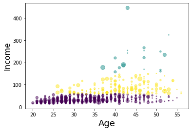
area = np.pi * ( X[:, 1])**2
plt.scatter(X[:, 0], X[:, 3], s=area, c=labels.astype(np.float), alpha=0.5)<br>
plt.xlabel('Age', fontsize=18)
plt.ylabel('Income', fontsize=16)
plt.show()

area = np.pi * ( X[:, 1])**2
plt.scatter(X[:, 1], X[:, 3], s=area, c=labels.astype(np.float), alpha=0.5)<br>
plt.xlabel('Education', fontsize=18)
plt.ylabel('Income', fontsize=16)
plt.show()
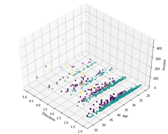
from mpl_toolkits.mplot3d import Axes3D
fig = plt.figure(1, figsize=(8, 6))
plt.clf()
ax = Axes3D(fig, rect=[0, 0, .95, 1], elev=48, azim=134)
plt.cla()
ax.set_xlabel('Education')
ax.set_ylabel('Age')
ax.set_zlabel('Income')
ax.scatter(X[:, 1], X[:, 0], X[:, 3], c= labels.astype(np.float))
Thus we find three categories of the cluster:
1-AFFLUENT, EDUCATED AND OLD AGED
2-MIDDLE AGED AND MIDDLE INCOME
3-YOUNG AND LOW INCOME
Hierarchical-based clustering
Hierarchical based clustering is divided into two categories:
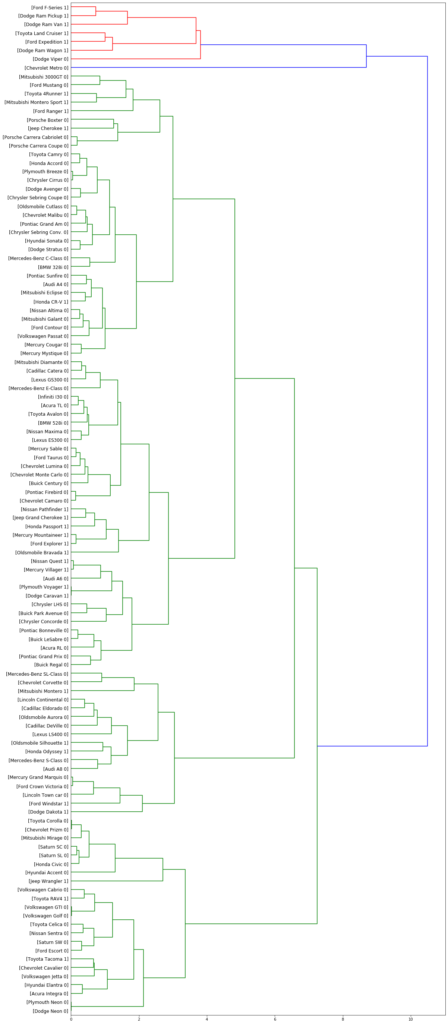
- Agglomerative: This is a “bottom-up” approach: each observation starts in its own cluster, and pairs of clusters are merged as one moves up the hierarchy.
- Divisive: This is a “top-down” approach: all observations start in one cluster, and splits are performed recursively as one moves down the hierarchy.
In agglomerative clustering we merge clusters. But, how can we calculate the distance between clusters when there are multiple points in each cluster? We can use different criteria to find the closest clusters and merge them.
There are different ways to calculate the distances of the cluster:
- Single Linkage Clustering.
- The minimum distance between clusters.
- Complete Linkage Clustering.
- The maximum distance between clusters.
- Average Linkage Clustering.
- The average distance between clusters.
- Centroid Linkage Clustering.
- Distance between cluster centroids.
In Hierarchical clustering, we don’t need a number of clusters to be defined so it’s easy to implement. but it is slow for large datasets and it always generates the same cluster.

Density-based clustering algorithms
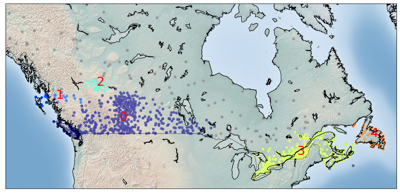
Density-based clustering algorithms locate regions of high density that are separated from one another by regions of low density. Density-based clustering algorithms are proper for arbitrary shape clusters. It works on two parameters, 1-radius and 2-minimum points
from sklearn.cluster import DBSCAN
import sklearn.utils
from sklearn.preprocessing import StandardScaler
sklearn.utils.check_random_state(1000)
Clus_dataSet = df[['lat','long']]
Clus_dataSet = np.nan_to_num(Clus_dataSet)
Clus_dataSet = StandardScaler().fit_transform(Clus_dataSet)
db = DBSCAN(eps=0.15, min_samples=10).fit(Clus_dataSet)
core_samples_mask = np.zeros_like(db.labels_, dtype=bool)
core_samples_mask[db.core_sample_indices_] = True
labels = db.labels_
df["Clus_Db"]=labels
realClusterNum=len(set(labels)) - (1 if -1 in labels else 0)
clusterNum = len(set(labels))
