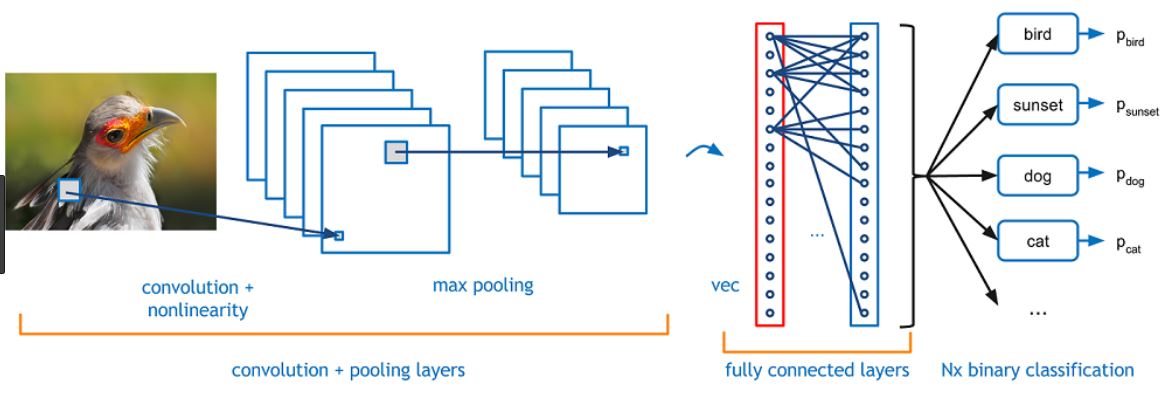
When we enter into the world of computer vision we have to understand how a computer understands an image. A colored image has three channels and a 2D data in each channel. When the image size increases Machine learning start suffering from the curse of dimensionality, in order to overcome from this Deep learning comes up with a special type of Feedforward neural network known as CNN- Convolutional Neural Network.
I hope a lot of videos is available on this so I am quickly jumping on the coding part…
Let’s start with MNIST dataset…
Here I will do the code using three ways, using simple Multiple perceptrons, then with Conv1D and with Conv2D. The default is 2D for images but could be 1D such as for words in a sentence or 3D for the video that adds a time dimension.
Multiple perceptrons
Import the libraries,
import numpy as np
from keras.models import Sequential
from keras.layers import Dense
from keras.utils import np_utils
from keras.datasets import mnist
Load data,
#  Load pre-shuffled MNIST data into train and test sets
import matplotlib.pyplot as plt
%matplotlib inline
(X_train, y_train), (X_test, y_test) = mnist.load_data()
plt.imshow(X_train[0])

num_pixels = X_train.shape[1] * X_train.shape[2]
X_train = X_train.reshape(X_train.shape[0], num_pixels).astype('float32')
X_test = X_test.reshape(X_test.shape[0], num_pixels).astype('float32')
X_train = X_train / 255
X_test = X_test / 255

y_train = np_utils.to_categorical(y_train)
y_test = np_utils.to_categorical(y_test)
num_classes = y_test.shape[1]
Now Create a model in Deep learning using Keras,
def baseline_model():
    model = Sequential()
    model.add(Dense(num_pixels, input_dim=num_pixels, kernel_initializer='normal',
    activation='relu'))
    model.add(Dense(num_classes, kernel_initializer='normal', activation='softmax'))
    model.compile(loss='categorical_crossentropy', optimizer='adam', metrics=['accuracy'])
    return model
Now Build and run the model.
#build the model
model = baseline_model()
# Fit the model
model.fit(X_train, y_train, validation_data=(X_test, y_test), epochs=10, batch_size=200,
verbose=2)
# Final evaluation of the model
scores = model.evaluate(X_test, y_test, verbose=0)
print("Baseline Error: %.2f%%" % (100-scores[1]*100))
Train on 60000 samples, validate on 10000 samples
Epoch 1/10
6s - loss: 0.2742 - acc: 0.9231 - val_loss: 0.1382 - val_acc: 0.9597
Epoch 2/10
4s - loss: 0.1097 - acc: 0.9682 - val_loss: 0.0985 - val_acc: 0.9701
Epoch 3/10
4s - loss: 0.0708 - acc: 0.9793 - val_loss: 0.0745 - val_acc: 0.9766
Epoch 4/10
4s - loss: 0.0500 - acc: 0.9849 - val_loss: 0.0660 - val_acc: 0.9795
Epoch 5/10
4s - loss: 0.0349 - acc: 0.9903 - val_loss: 0.0667 - val_acc: 0.9796
Epoch 6/10
4s - loss: 0.0273 - acc: 0.9926 - val_loss: 0.0599 - val_acc: 0.9819
Epoch 7/10
4s - loss: 0.0205 - acc: 0.9946 - val_loss: 0.0567 - val_acc: 0.9828
Epoch 8/10
4s - loss: 0.0137 - acc: 0.9970 - val_loss: 0.0570 - val_acc: 0.9823
Epoch 9/10
4s - loss: 0.0103 - acc: 0.9979 - val_loss: 0.0579 - val_acc: 0.9814
Epoch 10/10
5s - loss: 0.0085 - acc: 0.9982 - val_loss: 0.0621 - val_acc: 0.9809
Baseline Error: 1.91%
Conv1D
Import the libraries,
from keras.preprocessing import sequence
from keras.models import Sequential
from keras.layers import Dense, Dropout, Activation
from keras.layers import Embedding
from keras.layers import Conv1D, GlobalMaxPooling1D
from keras.datasets import imdb
Load Data,
#  Load pre-shuffled MNIST data into train and test sets
import matplotlib.pyplot as plt
%matplotlib inline
(X_train, y_train), (X_test, y_test) = mnist.load_data()
# set parameters:
max_features = 5000
maxlen = 784
batch_size = 32
embedding_dims = 50
filters = 250
kernel_size = 3
hidden_dims = 250
epochs = 2
num_pixels = X_train.shape[1] * X_train.shape[2]
#num_pixels 28*28=784
num_pixels = X_train.shape[1] * X_train.shape[2]
#num_pixels 28*28=784
X_train = X_train.reshape(X_train.shape[0],num_pixels).astype('float32')
X_test = X_test.reshape(X_test.shape[0],num_pixels).astype('float32')
X_train.shape
(60000, 784)
X_train = X_train / 255
X_test = X_test / 255
y_train = np_utils.to_categorical(y_train)
y_test = np_utils.to_categorical(y_test)
num_classes = y_test.shape[1]
y_train.shape
(60000, 10)
print('x_train shape:', X_train.shape)
print('x_test shape:', X_test.shape)
print('Build model...')
model = Sequential()
model.add(Embedding(max_features,
                    embedding_dims,
                    input_length=maxlen))
model.add(Conv1D(filters,
                 kernel_size,
                 padding='valid',
                 activation='relu',
                 strides=1))
# we use max pooling:
model.add(GlobalMaxPooling1D())
# We project onto a single unit output layer, and squash it with a sigmoid:
model.add(Dense(10))
model.add(Activation('softmax'))
model.compile(loss='categorical_crossentropy',
              optimizer='adam',
              metrics=['accuracy'])
model.fit(X_train, y_train,
          batch_size=batch_size,
          epochs=epochs,
          validation_data=(X_test, y_test))
Conv2D
Load Libraries,
#But this is not CNN its simple multi perceptron that are working as a CNN classifier
from keras.datasets import mnist
from keras.models import Sequential
from keras.layers import Dense
from keras.layers import Dropout
from keras.layers import Flatten
from keras.layers.convolutional import Conv2D
from keras.layers.convolutional import MaxPooling2D
from keras.utils import np_utils
from keras import backend as K
K.set_image_dim_ordering('th')
import matplotlib.pyplot as plt
(X_train, y_train), (X_test, y_test) = mnist.load_data()
%matplotlib inline
plt.imshow(X_train[0])
import numpy
# fix random seed for reproducibility
seed = 7
numpy.random.seed(seed)
# load data
(X_train, y_train), (X_test, y_test) = mnist.load_data()
# reshape to be [samples][channels][width][height]
X_train = X_train.reshape(X_train.shape[0], 1, 28, 28).astype('float32')
X_test = X_test.reshape(X_test.shape[0], 1, 28, 28).astype('float32')
# normalize inputs from 0-255 to 0-1
X_train = X_train / 255
X_test = X_test / 255
# one hot encode outputs
y_train = np_utils.to_categorical(y_train)
y_test = np_utils.to_categorical(y_test)
num_classes = y_test.shape[1]
plt.imshow(X_train[2232,0,:,:])

def baseline_model():
# create model
    model = Sequential()
    model.add(Conv2D(32, (5, 5), input_shape=(1, 28, 28), activation='relu'))
    model.add(MaxPooling2D(pool_size=(2, 2)))
    model.add(Dropout(0.2))
    model.add(Flatten())
    model.add(Dense(128, activation='relu'))
    model.add(Dense(num_classes, activation='softmax'))
    # Compile model
    model.compile(loss='categorical_crossentropy', optimizer='adam', metrics=['accuracy'])
    return model
model = baseline_model()
# Fit the model
model.fit(X_train, y_train, validation_data=(X_test, y_test), epochs=10, batch_size=200)
# Final evaluation of the model
scores = model.evaluate(X_test, y_test, verbose=0)
print("CNN Error: %.2f%%" % (100-scores[1]*100))
output:
Train on 60000 samples, validate on 10000 samples
Epoch 1/10
60000/60000 [==============================] - 75s - loss: 0.2322 - acc: 0.9341 - val_loss: 0.0817 - val_acc: 0.9745
Epoch 2/10
60000/60000 [==============================] - 75s - loss: 0.0738 - acc: 0.9781 - val_loss: 0.0466 - val_acc: 0.9841
Epoch 3/10
60000/60000 [==============================] - 75s - loss: 0.0533 - acc: 0.9839 - val_loss: 0.0433 - val_acc: 0.9860
Epoch 4/10
60000/60000 [==============================] - 75s - loss: 0.0401 - acc: 0.9877 - val_loss: 0.0405 - val_acc: 0.9871
Epoch 5/10
60000/60000 [==============================] - 75s - loss: 0.0338 - acc: 0.9893 - val_loss: 0.0347 - val_acc: 0.9877
Epoch 6/10
60000/60000 [==============================] - 75s - loss: 0.0275 - acc: 0.9913 - val_loss: 0.0303 - val_acc: 0.9897
Epoch 7/10
60000/60000 [==============================] - 75s - loss: 0.0233 - acc: 0.9926 - val_loss: 0.0345 - val_acc: 0.9885
Epoch 8/10
60000/60000 [==============================] - 75s - loss: 0.0204 - acc: 0.9937 - val_loss: 0.0322 - val_acc: 0.9888
Epoch 9/10
60000/60000 [==============================] - 74s - loss: 0.0166 - acc: 0.9946 - val_loss: 0.0300 - val_acc: 0.9901
Epoch 10/10
60000/60000 [==============================] - 74s - loss: 0.0146 - acc: 0.9957 - val_loss: 0.0316 - val_acc: 0.9899
CNN Error: 1.01%
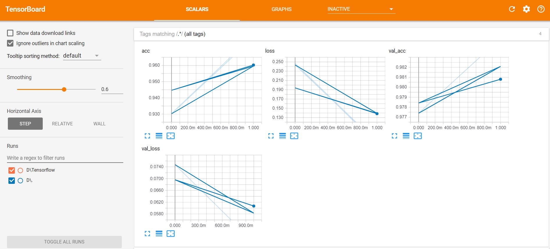
So we have 98% accuracy.
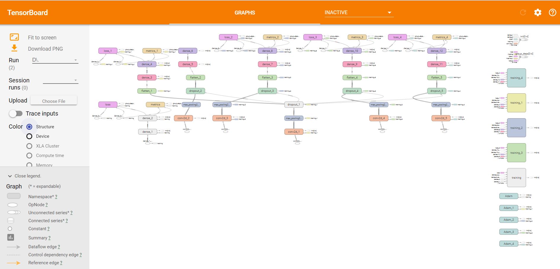
You can check it on tensorboard as well..
Hope this will help you a lot in order to understand a CNN.