Distributions

A distribution in statistics is a function that shows the possible values for a variable and how often they occur.

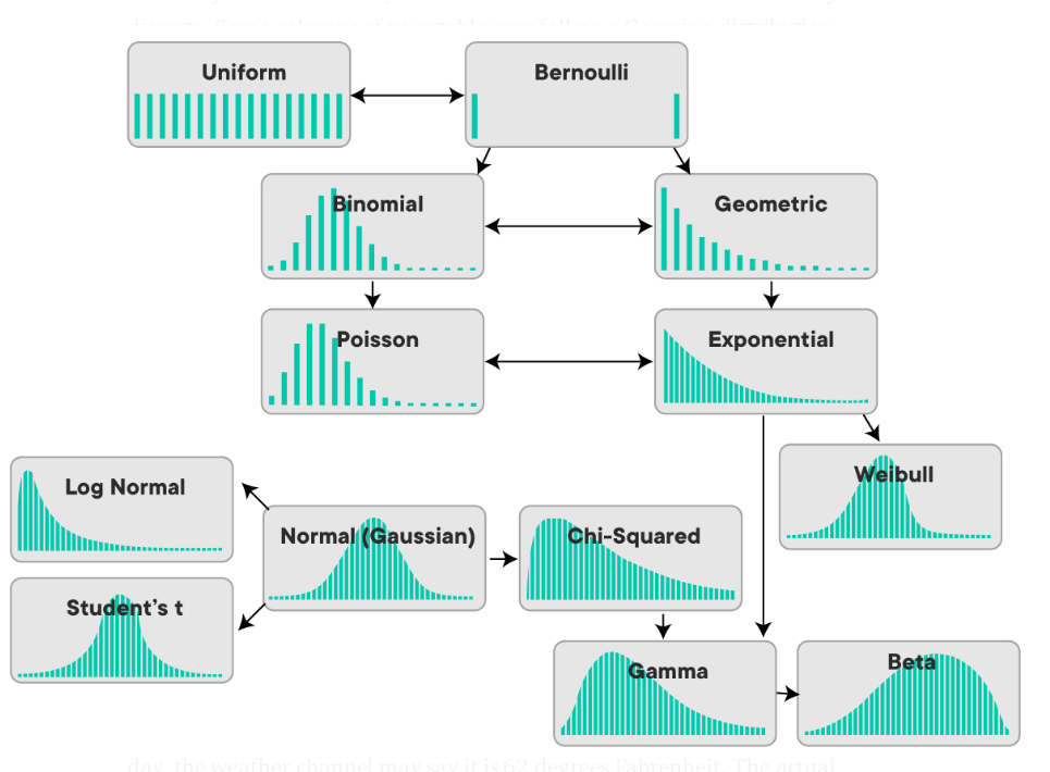
There are various distribution but the major distribution used in data science are :

1. Bernoulli Distribution
2. Uniform Distribution
3. Binomial Distribution
4. Normal Distribution
5. Poisson Distribution
6. Exponential Distribution

Family of Distribution

Parameterized families of distributions are the normal distributions, the Poisson distributions, the binomial distributions, and the exponential family of distributions. The family of normal distribution has two parameters, the mean and the variance: if those are specified, the distribution is known exactly.

Chi-squared families of distributions have one parameter: the number of degrees of freedom.

Nonparametric statistics is the branch of statistics that is not based solely on parametrized families of probability distributions (common examples of parameters are the mean and variance). Nonparametric statistics are based on either being distribution-free or having a specified distribution but with the distribution’s parameters unspecified. Nonparametric statistics include both descriptive statistics and statistical inference.

Bernoulli Distribution is a case of binomial distribution where we conduct a single experiment. It is a case of binomial distribution where we conduct a single experiment. This is a discrete probability distribution with probability p for value 1 and probability q=1-p for value 0.

from scipy.stats import bernoulli
data_bernoulli = bernoulli.rvs(p=0.8,loc=0,size=100)
ax = sb.distplot(data_bernoulli,kde=True,hist_kws={"linewidth": 15,'alpha':.35})
ax.set(xlabel='Binomial', ylabel='Frequency')

Binomial distribution tells us the probability of how often there will be a success in n independent experiments. Such experiments are yes-no questions. One example may be tossing a coin.

from scipy.stats import binom<br>
data_binom = binom.rvs(n=100,p=0.8,loc=0,size=100)<br>
ax = sb.distplot(data_binom,kde=True,hist_kws={"linewidth": 15,'alpha':.35})<br>
ax.set(xlabel='Binomial', ylabel='Frequency')

Uniform Distribution: When you roll a fair die, the outcomes are 1 to 6. The probabilities of getting these outcomes are equally likely and that is the basis of a uniform distribution. Unlike Bernoulli Distribution, all the n number of possible outcomes of a uniform distribution are equally likely.

from scipy.stats import uniform
data_uniform = uniform.rvs(loc=0, scale=1, size=1, random_state=None)
ax = sb.distplot(data_uniform,kde=True,hist_kws={"linewidth": 15,'alpha':.35})
ax.set(xlabel='Binomial', ylabel='Frequency')

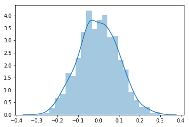
Normal Distribution: The normal distribution, also known as the Gaussian or standard normal distribution, is the probability distribution that plots all of its values in a symmetrical fashion, and most of the results are situated around the probability’s mean.

mu, sigma =0.5 , 0.1 # mean and standard deviation
x= np.random.normal(mu,sigma,1000)
sns.distplot(x)
print(np.mean(x))
print('Mean',np.mean(x))
print('Variance',np.var(x))
print('Skewness',(scipy.stats.skew(x)))
print('Kurtosis',scipy.stats.kurtosis(x))

0.499509404711
Mean 0.499509404711
Variance 0.0100355041263
Skewness 0.015929115377171493
Kurtosis 0.18598219816295503

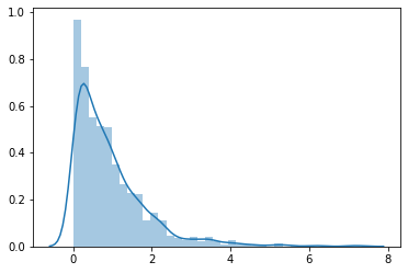
Exponential Distribution: It  (also known as a negative exponential distribution) is the probability distribution that describes the time between events in a Poisson point process, i.e. a process in which events occur continuously and independently at a constant average rate.

x=np.random.exponential(1,1000)
sb.distplot(x)
print('Mean',np.mean(x))
print('Variance',np.var(x))
print('Skewness',(scipy.stats.skew(x)))
print('Kurtosis',scipy.stats.kurtosis(x))

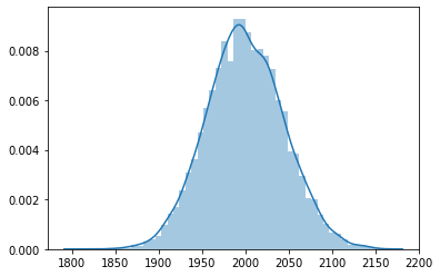
Poisson Distribution: The Poisson distribution is the limit of the binomial distribution for large N.

x = np.random.poisson(2000,10000) 
sb.distplot(x) 
print('Mean',np.mean(x))
print('Variance',np.var(x)) 
print('Skewness',(scipy.stats.skew(x))) 
print('Kurtosis',scipy.stats.kurtosis(x))

Refer : Analytics vidya