A Classical way, Logistic Regression is the younger son of Mr.ML, he is very efficient in predicting any problem associated with binary values. Whenever any person comes to Mr.ML and having problems like will his loan approves or not?, is it possible that he gets profit this year or not?, usually he asks his son Logistic to answer those question. Logistic plays with True/False or 0/1.

One Day a person came and told that he is using a mail system in his office and every day he receives thousands of SMS but it is impossible for him to predict the ham or spam SMS. He asked him to collect a sample of SMS and give it to Logistic and he will prepare a model that will solve his problem.
After few days the person came with following sample data:
| Type | SMS | |
|---|---|---|
| 0 | ham | Go until jurong point, crazy.. Available only … |
| 1 | ham | Ok lar… Joking wif u oni… |
| 2 | spam | Free entry in 2 a wkly comp to win FA Cup fina… |
| 3 | ham | U dun say so early hor… U c already then say… |
| 4 | ham | Nah I don’t think he goes to usf, he lives aro… |
| 5 | spam | FreeMsg Hey there darling it’s been 3 week’s n… |
| 6 | ham | Even my brother is not like to speak with me. … |
| 7 | ham | As per your request ‘Melle Melle (Oru Minnamin… |
| 8 | spam | WINNER!! As a valued network customer you have… |
| 9 | spam | Had your mobile 11 months or more? U R entitle… |
Now Programmatically we can solve the problem like this,
Import the libraries:
import pandas as pd
from sklearn.linear_model.logistic import LogisticRegression
from sklearn.cross_validation import train_test_split
from sklearn.feature_extraction.text import TfidfVectorizer
Load the file,
df=pd.read_csv('SMSSpamCollection.csv',delimiter='\t',header=None)
X_train_raw, X_test_raw, y_train, y_test = train_test_split(df[1],df[0])
Vectorize it by using Term frequency-inverse document frequency(TFIDF)
vectorizer = TfidfVectorizer()
X_train = vectorizer.fit_transform(X_train_raw)
X_test = vectorizer.transform(X_test_raw)
Make a Model,
classifier = LogisticRegression()
classifier.fit(X_train, y_train)
Now we may predict anything,
predictions = classifier.predict(X_test)

for i, prediction in enumerate(predictions[:5]):
    #print(X_test_raw[0])
    print('Prediction: %s. Message: %s'%(prediction, list(X_test_raw)[i]))
output is:
Prediction: ham. Message: My uncles in Atlanta. Wish you guys a great semester.
Prediction: ham. Message: I wanted to wish you a Happy New Year and I wanted to talk to you about some legal advice to do with when Gary and I split but in person. I'll make a trip to Ptbo for that. I hope everything is good with you babe and I love ya :)
Prediction: ham. Message: Fighting with the world is easy, u either win or lose bt fightng with some1 who is close to u is dificult if u lose - u lose if u win - u still lose.
Prediction: ham. Message: Honestly i've just made a lovely cup of tea and promptly dropped my keys in it and then burnt my fingers getting them out!
Prediction: spam. Message: 85233 FREE>Ringtone!Reply REAL
The Hypothesis function is hθ(x) = g((θT x))
However, some other assumptions that we have to consider before going with this approach.
1-Binary logistic regression requires the dependent variable to be binary and ordinal logistic regression requires the dependent variable to be ordinal.
Note: Cardinal: how many, Ordinal: position, Nominal: name
2-Logistic regression requires the observations to be independent of each other.
3-Logistic regression requires there to be little or no multicollinearity among the independent variables.
4-Logistic regression typically requires a large sample size because it works on probability. For example, if you have 5 independent variables and the expected probability of your least frequent outcome is .10, then you would need a minimum sample size of 500 (10*5 / .10).
In order to find the correctness of the model logistic uses matrices. The most common metrics are accuracy, precision, recall, F1 measure, and ROC AUC score. All of these measures depend on the concepts of true positives, true negatives, false positives, and false negatives. Positive and negative refer to the classes. True and false denote whether the predicted class is the same as the true class.
As an example,
- correctly identified “good” person(true positive);
- “good” person, mistakenly identified as “bad” ones (False Negative);
- “bad” person mistakenly identified as “good” ones (False Positive);
- correctly identified “bad” people (True Negative).
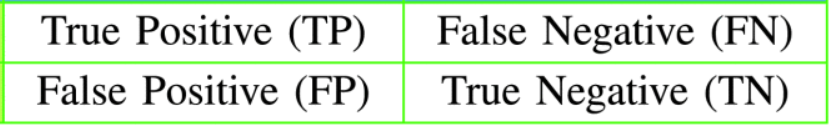
A confusion matrix, or contingency table, can be used to visualize true and false positives and negatives. The rows of the matrix are the true classes of the instances, and the columns are the predicted classes of the instances:
from sklearn.metrics import confusion_matrix
import matplotlib.pyplot as plt
y_test = [0, 0, 0, 0, 0, 1, 1, 1, 1, 1]
y_pred = [0, 1, 0, 0, 0, 0, 0, 1, 1, 1]
confusion_matrix = confusion_matrix(y_test, y_pred)
print(confusion_matrix)
plt.matshow(confusion_matrix)
plt.title('Confusion matrix')
plt.colorbar()
plt.ylabel('True label')
plt.xlabel('Predicted label')
plt.show()
Output:
[[4 1]
 [2 3]]

Accuracy: Accuracy measures a fraction of the classifier’s predictions that are correct.
from sklearn.metrics import accuracy_score
y_pred, y_true = [0, 1, 1, 0], [1, 1, 1, 1]
print ('Accuracy:', accuracy_score(y_true, y_pred))
Output:0.5
Precision and recall: Precision is the fraction of positive predictions that are correct/true.
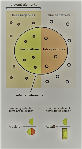
The F1: It measures is the harmonic mean, or weighted average, of the precision and recall scores. Also called the f-measure or the f-score, the F1 score is calculated using
the following formula:

ROC: A Receiver Operating Characteristic, ROC curves plot the classifier’s recall against its fall-out. Fall-out, or the false positive rate, is the number of false positives divided by the total number of negatives.
AUC: AUC is the area under the ROC curve; it reduces the ROC curve to a single value, which represents the expected performance of the classifier.
Thanks to:
Reference-Link
Reference –Link
Reference-Link