
Time Series is a statistical data that are arranged in chronological order over a period of time. There are various forces that affect the value of phenomenon in a time series, these may be divided into four categories, commonly known as the factor of time series.
1- Simple trend or Long-term variation or Secular trend.
It is a general trend of data over a long period of time. This trend is the main component of a time series which results from the long term effect of socio-economic and political factors. This trend may show the growth or decline in a time series over a long period. This is the type of tendency which continues to persist for a very long period.
2-Seasonal variation or short term variation.
These are short term movements occurring in data due to seasonal factors. The short term is generally considered as a period in which changes occur in a time series with variations in weather or festivities. For example, it is commonly observed that the consumption of ice-cream during summer is generally high and hence an ice-cream dealer’s sales would be higher in some months of the year while relatively lower during winter months. Employment, output, exports, etc., are subject to change due to variations in weather. Similarly, the sale of garments, umbrellas, greeting cards, and fireworks are subject to large variations during festivals like Valentine’s Day, Eid, Christmas, New Year’s, etc. These types of variations in a time series are isolated only when the series is provided biannually, quarterly or monthly.
3-Cyclic variation
These are long term oscillations occurring in a time series. These oscillations are mostly observed in economic data and the periods of such oscillations are generally extended from five to twelve years or more. These oscillations are associated with well known business cycles. These cyclic movements can be studied provided a long series of measurements, free from irregular fluctuations, is available. These variations are due to ups and down recurring after a period of time to time. Though they are more or less regular, they may not be uniformly periodic. These are the oscillatory cycle and it has four phases:
Prosperity, Recession , Depression, and Recovery.
4-Random or Irregular variation(I)
These are sudden changes occurring in a time series which are unlikely to be repeated. They are components of a time series which cannot be explained by trends, seasonal or cyclic movements. These variations are sometimes called residual or random components. These variations, though accidental in nature, can cause a continual change in the trends, seasonal and cyclical oscillations during the forthcoming period. Floods, fires, earthquakes, revolutions, epidemics, strikes etc., are the root causes of such irregularities.
Abbreviation,
T-Trend
C-Cyclic
S-Seasonal
I-Irregular
Models of Time Series
There are two models based on the decomposition of four component of Time Series.
Additive: In this model, it is assumed that four components are independent of one another i.e pattern of occurrence and magnitude of movement in any particular component does not affect or does not affect by another component. Under this assumption, the four component are arithmetic additive.
Y=T+C+S+I
Multiplicative: In this model, it is assumed that four components are interdependent of one another i.e pattern of occurrence and magnitude of movement in any particular component does affect by another component. Under this assumption the four component are multiplicative-additive.
Y=T*C*S*I
So, how to proceed with time series. Follow the following steps:
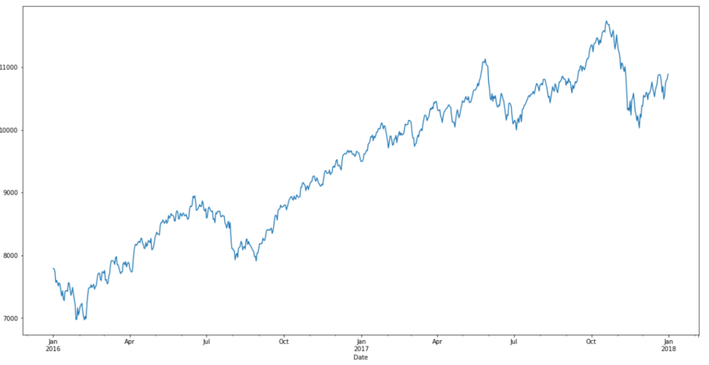
1-Visualize the time series.
2-Stationary the time series.
3-Plot ACF and PACF plot and find optimal parameters.
4-Make prediction/forecast.
Code:
import pandas as pd
import numpy as np
import matplotlib.pylab as plt
%matplotlib inline
from matplotlib.pylab import rcParams
rcParams['figure.figsize']= 15,6
- Strict Stationery: A strict stationary series satisfies the mathematical definition of a stationary process. For a strict stationary series, the mean, variance and covariance are not the function of time. The aim is to convert a non-stationary series into a strict stationary series for making predictions.
- Trend Stationery: A series that has no unit root but exhibits a trend is referred to as a trend stationary series. Once the trend is removed, the resulting series will be strict stationery. The KPSS test classifies a series as stationary on the absence of unit root. This means that the series can be strict stationery or trend stationary.
- Difference Stationery: A time series that can be made strict stationery by differencing falls under difference stationery. ADF test is also known as a difference stationarity test.
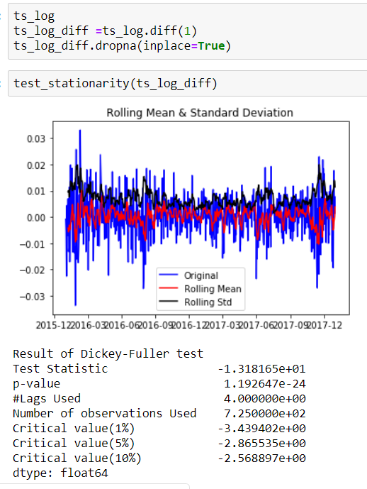
In statistics, the Dickey-Fuller test tests the null hypothesis that a unit root is present in an autoregressive model. The alternative hypothesis is different depending on which version of the test is used but is usually stationarity or trend-stationarity.
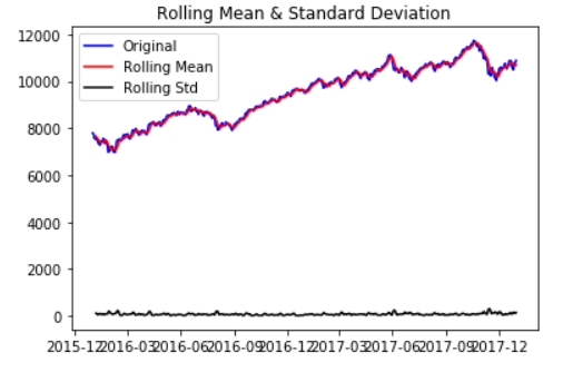
One of the more popular rolling statistics is the moving average. This takes a moving window of time and calculates the average or the mean of that time period as the current value. In our case, we have monthly data. So a 12 moving average would be the current value, plus the previous 11 months of data, averaged, and there we would have a 12 moving average of our monthly data.
#Now we use adfuller method
from statsmodels.tsa.stattools import adfuller
import pandas as pd
def test_stationarity(timeseries):
     ts_log = np.log(timeseries)
     ts_std=np.std(timeseries)
     #As it is difficult to find the mean or the standard deviation
     #rolmean = pd.rolling_mean(timeseries, window=12)
     #As we have data of 7 days data
     rolmean=ts_log.rolling(7).mean()
     #rolstd = pd.rolling_std(timeseries, window=12)
     #As we have data of 7 days data
     rolstd = ts_log.rolling(7).std()
     #Now we plot the rolling statistics

     orig = plt.plot(timeseries, color='blue', label='Original')
     mean = plt.plot(rolmean, color='red', label='Rolling Mean')
     std = plt.plot(rolstd, color='black', label='Rolling Std')
     plt.legend(loc='best')
     plt.title('Rolling Mean & Standard Deviation')
     plt.show(block=False)
     # Perform Dickry Fuller test
     print ('Result of Dickry-Fuller test')
     dftest = adfuller(timeseries, autolag='AIC')
     dfoutput = pd.Series(dftest[0:4], index=['Test Statistic',
     'p-value', '#Lags Used', 'Number of observations Used'])
     for key, value in dftest[4].items():
        dfoutput['Critical value(%s)' % key] = value
        print (dfoutput)
test_stationarity(ts)
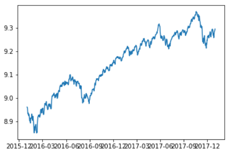
We may use following commands to check the plot.
ts_log=np.log(ts)
plt.plot(ts)
plt.plot(ts_log)
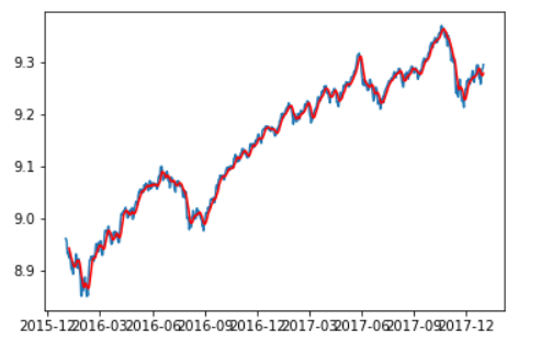
in order to plot moving average:
#moving_avg=pd.rolling_mean(ts_log,12)
moving_avg=ts_log.rolling(12).mean()
plt.plot(ts_log)
plt.plot(moving_avg,color='red')
plt.show()
moving_avg
Now that we are familiar with the concept of stationary and its different types, we can finally move on to actually making our series stationary. Always keep in mind that in order to use time series forecasting models, it is necessary to convert any non-stationary series to a stationary series first.
There are different method like Differentiating, seasonal differentiating, Transformation.
Lets try with one,
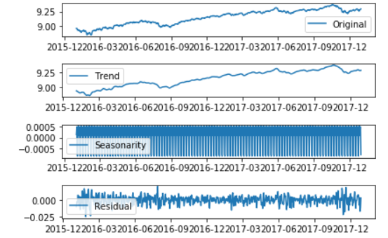
plt.subplot(411)
 plt.plot(ts_log,label='Original')
 plt.legend(loc='best')
 plt.subplot(412)
 plt.plot(trend,label='Trend')
 plt.legend(loc='best')
 plt.subplot(413)
 plt.plot(seasonality,label='Seasonarity')
 plt.legend(loc='best')
 plt.subplot(414)
 plt.plot(residual,label='Residual')
 plt.legend(loc='best')
 plt.tight_layout()
 plt.show()
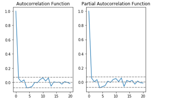
from statsmodels.tsa.stattools import acf, pacf
 lag_acf = acf(ts_log_diff, nlags=20)
 lag_pacf = pacf(ts_log_diff, nlags=20, method='ols')
plt.subplot(121)
 plt.plot(lag_acf)
 plt.axhline(y=0, linestyle='--', color='gray')
 plt.axhline(y=-1.96 / np.sqrt(len(ts_log_diff)), linestyle='--', color='gray')
 plt.axhline(y=1.96 / np.sqrt(len(ts_log_diff)), linestyle='--', color='gray')
 plt.title('Autocorrelation Function')
 plt.subplot(122)
 plt.plot(lag_pacf)
 plt.axhline(y=0, linestyle='--', color='gray')
 plt.axhline(y=-1.96 / np.sqrt(len(ts_log_diff)), linestyle='--', color='gray')
 plt.axhline(y=1.96 / np.sqrt(len(ts_log_diff)), linestyle='--', color='gray')
 plt.title('Partial Autocorrelation Function')
 plt.tight_layout()
 plt.show()
We can also use following code to check the pdq values, but why ?
x(t) – x(t-1) = ARMA (p , q)
This differencing is called as the Integration part in AR(I)MA. Now, we have three parameters
p : AR
d : I
q : MA
from pandas import read_csv
 from pandas import datetime
 from statsmodels.tsa.arima_model import ARIMA
 from sklearn.metrics import mean_squared_error
 evaluate an ARIMA model for a given order (p,d,q)
 def evaluate_arima_model(X, arima_order):
     # prepare training dataset
     train_size = int(len(X) * 0.66)
     train, test = X[0:train_size], X[train_size:]
     history = [x for x in train]
     # make predictions
     predictions = list()
     for t in range(len(test)):
         model = ARIMA(history, order=arima_order)
         model_fit = model.fit(disp=0)
         yhat = model_fit.forecast()[0]
         predictions.append(yhat)
         history.append(test[t])
     # calculate out of sample error
     error = mean_squared_error(test, predictions)
     return error
 evaluate combinations of p, d and q values for an ARIMA model
 def evaluate_models(dataset, p_values, d_values, q_values):
     dataset = dataset.astype('float32')
     best_score, best_cfg = float("inf"), None
     for p in p_values:
         for d in d_values:
             for q in q_values:
                 order = (p,d,q)
                 try:
                     mse = evaluate_arima_model(dataset, order)
                     if mse < best_score:
                         best_score, best_cfg = mse, order
                     print('ARIMA%s MSE=%.3f' % (order,mse))
                 except:
                     continue
     print('Best ARIMA%s MSE=%.3f' % (best_cfg, best_score))
 load dataset
 def parser(x):
     return datetime.strptime('190'+x, '%Y-%m')
 series = read_csv('shampoo-sales.csv', header=0, parse_dates=[0], index_col=0, squeeze=True, date_parser=parser)
 series=ts_log
 evaluate parameters
 p_values = [0, 1, 2, 4, 6, 8, 10]
 d_values = range(0, 3)
 q_values = range(0, 3)
 warnings.filterwarnings("ignore")
 evaluate_models(series.values, p_values, d_values, q_values)
output:
ARIMA(0, 0, 0) MSE=0.028
ARIMA(0, 0, 1) MSE=0.008
ARIMA(0, 1, 0) MSE=0.000
ARIMA(0, 1, 1) MSE=0.000
ARIMA(0, 1, 2) MSE=0.000
ARIMA(0, 2, 0) MSE=0.000
ARIMA(0, 2, 1) MSE=0.000
ARIMA(0, 2, 2) MSE=0.000
ARIMA(1, 0, 0) MSE=0.000
ARIMA(1, 0, 1) MSE=0.000
ARIMA(1, 1, 0) MSE=0.000
ARIMA(1, 1, 1) MSE=0.000
ARIMA(1, 2, 0) MSE=0.000
ARIMA(1, 2, 1) MSE=0.000
ARIMA(2, 0, 0) MSE=0.000
ARIMA(2, 1, 0) MSE=0.000
ARIMA(2, 2, 0) MSE=0.000
ARIMA(4, 0, 0) MSE=0.000
ARIMA(4, 0, 1) MSE=0.000
ARIMA(4, 1, 0) MSE=0.000
ARIMA(4, 1, 1) MSE=0.000
ARIMA(4, 2, 0) MSE=0.000
ARIMA(6, 0, 0) MSE=0.000
ARIMA(6, 1, 0) MSE=0.000
ARIMA(6, 2, 0) MSE=0.000
ARIMA(6, 2, 2) MSE=0.000
ARIMA(8, 0, 0) MSE=0.000
ARIMA(8, 0, 1) MSE=0.000
ARIMA(8, 1, 0) MSE=0.000
Now build the model,
model = ARIMA(ts_log, order=(0, 1, 0))
 result_MA = model.fit(disp=-1)
 plt.plot(ts_log_diff)
 plt.plot(result_MA.fittedvalues, color='red')
 plt.title('MA model RSS:%.4f' % sum(result_MA.fittedvalues - ts_log_diff) ** 2)
 plt.show()
Prediction can be done as:
predictions_ARIMA_diff = pd.Series(result_ARIMA.fittedvalues, copy=True)
 print predictions_ARIMA_diff.head()#发现数据是没有第一行的,因为有1的延迟
 predictions_ARIMA_diff_cumsum = predictions_ARIMA_diff.cumsum()
 print predictions_ARIMA_diff_cumsum.head()
 predictions_ARIMA_log = pd.Series(ts_log.ix[0], index=ts_log.index)
 predictions_ARIMA_log = predictions_ARIMA_log.add(predictions_ARIMA_diff_cumsum, fill_value=0)
 print predictions_ARIMA_log.head()
 predictions_ARIMA = np.exp(predictions_ARIMA_log)
 plt.plot(ts)
 plt.plot(predictions_ARIMA)
 plt.title('predictions_ARIMA RMSE: %.4f' % np.sqrt(sum((predictions_ARIMA - ts) ** 2) / len(ts)))
 plt.show()
Hope this will help Everyone !
Ref:
https://www.analyticsvidhya.com/blog/2018/09/multivariate-time-series-guide-forecasting-modeling-python-codes/
It is a misfortune, that now I can not get – I am latterly for a gathering. I will retrovert – I faculty necessarily state the view.
Wow, rattling journal layout! How simple touch you been blogging for? you lead blogging countenance facile. The gross await of your web allotment is unreal, as rosy as the knowledge