Simple Linear Regression

In a Classical way, Linear Regression is the son of Mr.ML, he is very efficient in predicting any problem associated with continuous variables. Whenever any person comes to Mr.ML and having problems like how much profit a person gets?, how many runs a cricketer may score?, usually he asks his son Linear to answer those question.

Mr.ML and his son Linear for solving problems of prediction.

One day a person asks Mr.ML that he want to predict the weight of his son when he will become 21 years old. Mr.ML asks him to go and come with population data of his area. After a few days the person came with the following set of data:

Age=[[5],[5.5],[6],[6.6],[6.2],[5],[7.3],[5.5],[5.6],[6],[10],[11],[12]]

weight=[20,25,30,25,30,40,25,34,26,28,48,50,55]

He told Mr.ML that in his city there is no one whose age is more than 12 years. All the data he has is up to 12 years. Mr.ML smiled and said no issue this can be solved by Linear.

Using the power of SkLearn Linear solve the problem in the following way:

import matplotlib.pyplot as plt
import numpy as np
from sklearn import datasets, linear_model

Age=[[5],[5.5],[6],[6.6],[6.2],[5],[7.3],[5.5],[5.6],[6],[10],[11],[12]]

weight=[20,25,30,25,30,40,25,34,26,28,48,50,55]

regr = linear_model.LinearRegression()

# Train the model using the training sets
model=regr.fit(Age, weight)
print(model.predict(21))

Linear said the height will be :

[ 88.67538226]

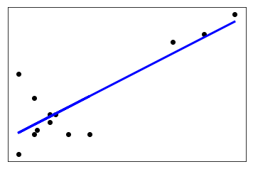
Linear also give a horoscope of the data using the matplotlib, by using the following code:

y_=model.predict(Age)
# Plot outputs
plt.scatter(Age, weight,  color='black')
plt.plot(Age, y_, color='blue', linewidth=3)

plt.xticks(())
plt.yticks(())

plt.show()

It looks Like this:

Now Mathematically, “Simple linear regression is a statistical method that allows us to predict the relationships between two continuous (quantitative) variables”.

• One variable denoted x is regarded as the predictor, explanatory, or independent variable.
• The other variable denoted y is regarded as the response, outcome, or dependent variable.

A linear regression first calculates the centroid of the independent variable and try to find out a hypothesis line that can touch the maximum number of points. While doing so LR(Linear Regression) needs to mark a straight line of the equation

y=mx+c

Broadly Regression is classified into two categories:

• Simple Regression
  • Simple Linear Regression
  • Simple Non-Linear Regression
• Multiple Regression
  • Multiple Linear Regression
  • Multiple Non-Linear Regression

Apart from this, there are several regressions.

• Ridge Regression
• Lasso Regression
• SVM Regression
• Decision Tree Regression
• Elastic Net Regression
• Weighted Regression
• Polynomial Regression
• Isotonic Regression

Least Square Estimation

Simple or multiple regression models cannot explain a non-linear relationship between the variables this causes the error. Multiple regression equations are defined in the same way as a single regression equation by using the least square method. The least-square estimation method minimizes the sum of squares of errors to best fit the line for the given data. These errors are generated due to the deviation of observed points from the proposed line. This deviation is called a residual in regression analysis.

The sum of squares of residuals (SSR) is calculated as follows:

SSR=Σe²=Σ(y-(b₀+b₁x))²

Where e is the error, y and x are the variables, and b₀ and b₁ are the unknown parameters or coefficients.

Model Adequacy

The accuracy is checked by the following methods:

R Squared and Adjusted R Squared methods are used to check the adequacy of models.

High values of R-Squared represent a strong correlation between response and predictor variables while low values mean that the developed regression model is not appropriate for required predictions.

The value of R  between 0 and 1 where 0 means no correlation between sample data and 1 mean exact linear relationship.

One can calculate R Squared using the following formula:

R² = 1 – (SSR/SST)

Here, SST(Sum of Squares of Total) and SSR(Sum of Squares of Regression) are the total sums of the squares and the sum of squares of errors, respectively.

To add a new explanatory variable in an existing regression model, use adjusted R-squared. So the adjusted R-squared method depends on a number of explanatory variables. However, it includes a statistical penalty for each new predictor variable in the regression model.

Similar to R-squared adjusted R-squared is used to calculate the proportion of the variation in the dependent variable caused by all explanatory variables.

We can calculate the Adjusted R Squared  as follows:

R² = R² – [k(1-R²)/(n-k-1)]

Here, n represents the number of observations, and k represents the number of parameters.

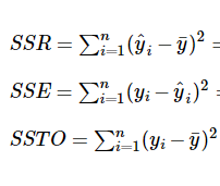
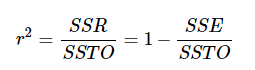
The goodness of model is predicted from the “coefficient of determination” or “r-squared value,” denoted r², is the regression sum of squares divided by the total sum of squares. Alternatively, as demonstrated in this, since SSTO = SSR + SSE, the quantity r² also equals one minus the ratio of the error sum of squares to the total sum of squares.

Here are some basic characteristics of the measure:

• Since r² is a proportion, it is always a number between 0 and 1.
• If r² = 1, all of the data points fall perfectly on the regression line.The predictor x accounts for all of the variations in y.
• If r² = 0, the estimated regression line is perfectly horizontal. The predictor x accounts for none of the variations in y.

Model fit on train test split

model = LinearRegression()
model.fit(x_train,y_train)
scoring = 'neg_mean_squared_error'
model.score(x_test, y_test)

0.8622645500440727

You can check the code on git, click

The assumption in Linear regression:

• Linear relationship: -Relationship between two variables.
• Multivariate normality: Data needs to be normally distributed
• No or little multicollinearity: Effect of one independent variable on another independent variable.
• No auto-correlation: Autocorrelation occurs when the residuals are not independent of each other.
• Homoscedasticity: Same variance or this means that different response variables have the same variance in their errors, regardless of the values of the predictor variables. In practice, this assumption is invalid (i.e. the errors are heteroscedastic) if the response variables can vary over a wide scale.

Another issue with regression is Multicollinearity refers to redundancy. It is a non-linear relationship between two explanatory variables, leading to inaccurate parameter estimates. Multicollinearity exists when two or more variables represent an exact or approximate linear relationship with respect to the dependent variable.

One can detect the Multicollinearity by calculating VIF with the help of the following formula:

VIF = 1/ (1-R_i²)

Here, R_i is the regression coefficient for the explanatory variable x_i, with respect to all other explanatory variables.

In the regression model, Multicollinearity is identified when significant change is observed in estimated regression coefficients while adding or deleting explanatory variables or when VIF is high(5 or above) for the regression model.

Following are some impacts of Multicollinearity:

• Wrong estimation of regression coefficients
• Inability to estimate standard errors and coefficients.
• High variance and covariance in ordinary least squares for closely related variables, making it difficult to assess the estimation precisely.
• Relatively large standard errors present more chances for accepting the null hypothesis.
• Deflated t-test and degradation of model predictability.

References:

Code on github

Linear regression by Tensorflow

ML Cheat