Linear Regression(TensorFlow)

It is one of the most widely known modeling technique. In this technique, the dependent variable is continuous, independent variable(s) can be continuous or discrete, and nature of regression line is linear.
Linear Regression establishes a relationship between dependent variable (Y) and one or more independent variables (X) using a best fit straight line (also known as regression line).

Linear regression can be implemented by varius techniques , but it can be visualized by tensorflow in a very different way.

#Import Libraies

import tensorflow as tf
import numpy
import matplotlib.pyplot as plt
rng = numpy.random

# Parameters
learning_rate = 0.01
training_epochs = 1000
display_step = 50

# Training Data
train_X = numpy.asarray([3.3,4.4,5.5,6.71,6.93,4.168,9.779,6.182,7.59,2.167,
7.042,10.791,5.313,7.997,5.654,9.27,3.1])
train_Y = numpy.asarray([1.7,2.76,2.09,3.19,1.694,1.573,3.366,2.596,2.53,1.221,
2.827,3.465,1.65,2.904,2.42,2.94,1.3])
n_samples = train_X.shape[0]

# tf Graph Input
X = tf.placeholder('float')
Y = tf.placeholder('float')

# Set model weights
W = tf.Variable(rng.randn(), name='weight')
b = tf.Variable(rng.randn(), name='bias')

# Construct a linear model
pred = tf.add(tf.multiply(X, W), b)

# Mean squared error
cost = tf.reduce_sum(tf.pow(pred-Y, 2))/(2*n_samples)
# Gradient descent
optimizer = tf.train.GradientDescentOptimizer(learning_rate).minimize(cost)

# Initializing the variables
init = tf.global_variables_initializer()

# Launch the graph
with tf.Session() as sess:
    sess.run(init)
    for epoch in range(training_epochs):
        for (x, y) in zip(train_X, train_Y):
            sess.run(optimizer, feed_dict={X: x, Y: y})

        # Display logs per epoch step
        if (epoch+1) % display_step == 0:
            c = sess.run(cost, feed_dict={X: train_X, Y:train_Y})
            print("Epoch:", '%04d' % (epoch+1), "cost=", "{:.9f}".format(c), \
                "W=", sess.run(W), "b=", sess.run(b))

    print("Optimization Finished!")
    
    training_cost = sess.run(cost, feed_dict={X: train_X, Y: train_Y})
    print("Training cost=", training_cost, "W=", sess.run(W), "b=", sess.run(b), '\n')
    
        # Graphic display
    plt.plot(train_X, train_Y, 'ro', label='Original data')
    plt.plot(train_X, sess.run(W) * train_X + sess.run(b), label='Fitted line')
    plt.legend()
    plt.show()

    # Testing example, as requested (Issue #2)
    test_X = numpy.asarray([6.83, 4.668, 8.9, 7.91, 5.7, 8.7, 3.1, 2.1])
    test_Y = numpy.asarray([1.84, 2.273, 3.2, 2.831, 2.92, 3.24, 1.35, 1.03])

    print("Testing... (Mean square loss Comparison)")
    testing_cost = sess.run(
        tf.reduce_sum(tf.pow(pred - Y, 2)) / (2 * test_X.shape[0]),
        feed_dict={X: test_X, Y: test_Y})  # same function as cost above
    print("Testing cost=", testing_cost)
    print("Absolute mean square loss difference:", abs(training_cost - testing_cost))

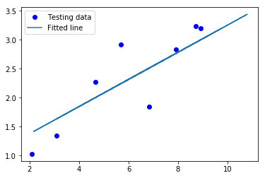
    plt.plot(test_X, test_Y, 'bo', label='Testing data')
    plt.plot(train_X, sess.run(W) * train_X + sess.run(b), label='Fitted line')
    plt.legend()
    plt.show()
    
    

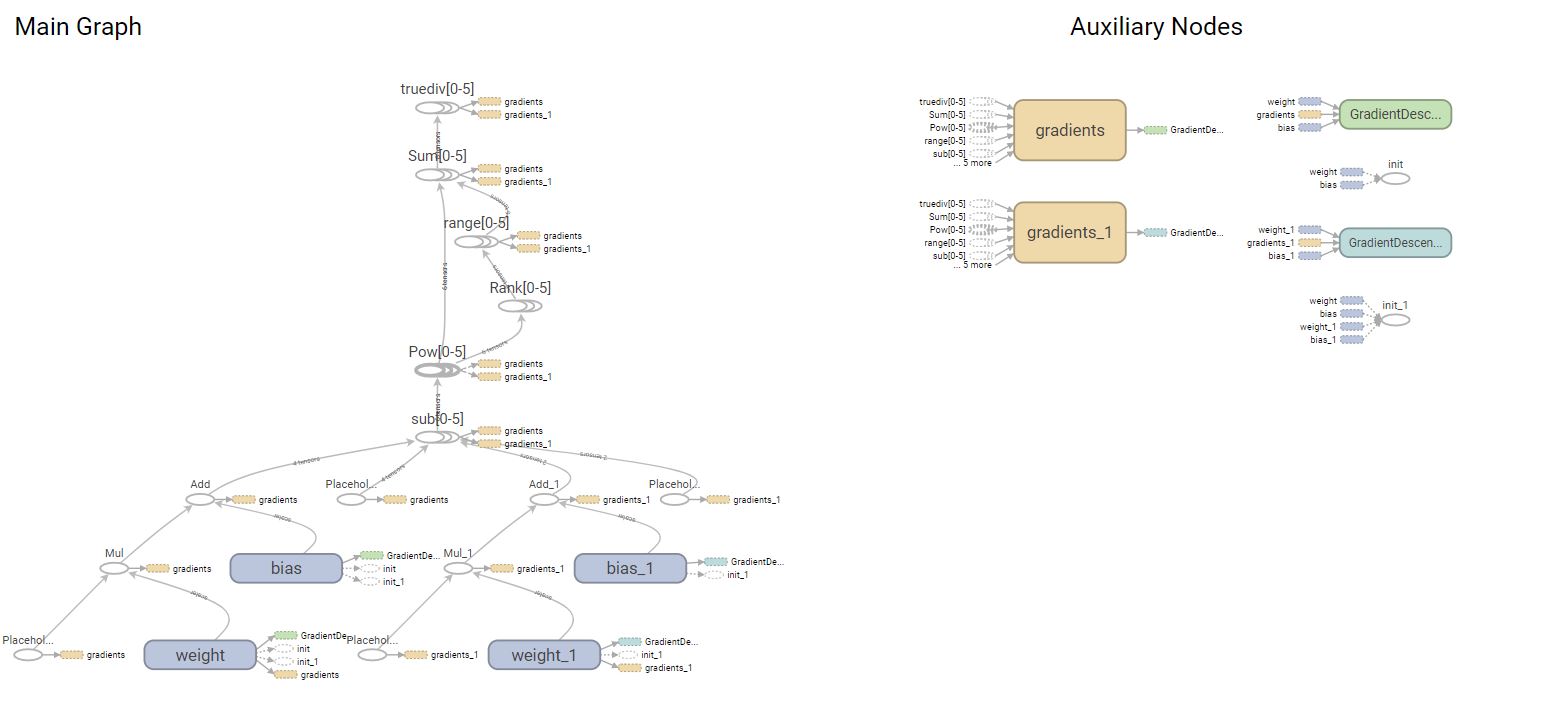
    writer= tf.summary.FileWriter('D:\Graph\Tensorflow',sess.graph)
    writer.close()
    sess.close()

Output:

Epoch: 0050 cost= 0.084654316 W= 0.200937 b= 1.1515
Epoch: 0100 cost= 0.083774000 W= 0.203831 b= 1.13068
Epoch: 0150 cost= 0.082994938 W= 0.206553 b= 1.1111
Epoch: 0200 cost= 0.082305610 W= 0.209113 b= 1.09268
Epoch: 0250 cost= 0.081695616 W= 0.21152 b= 1.07537
Epoch: 0300 cost= 0.081155792 W= 0.213784 b= 1.05908
Epoch: 0350 cost= 0.080678098 W= 0.215914 b= 1.04375
Epoch: 0400 cost= 0.080255359 W= 0.217917 b= 1.02935
Epoch: 0450 cost= 0.079881236 W= 0.219801 b= 1.01579
Epoch: 0500 cost= 0.079550095 W= 0.221573 b= 1.00304
Epoch: 0550 cost= 0.079257071 W= 0.223239 b= 0.991056
Epoch: 0600 cost= 0.078997687 W= 0.224807 b= 0.979779
Epoch: 0650 cost= 0.078768112 W= 0.226281 b= 0.969173
Epoch: 0700 cost= 0.078564890 W= 0.227668 b= 0.959197
Epoch: 0750 cost= 0.078385077 W= 0.228972 b= 0.949818
Epoch: 0800 cost= 0.078225911 W= 0.230198 b= 0.940996
Epoch: 0850 cost= 0.078085005 W= 0.231351 b= 0.932699
Epoch: 0900 cost= 0.077960268 W= 0.232436 b= 0.924895
Epoch: 0950 cost= 0.077849805 W= 0.233457 b= 0.917556
Epoch: 1000 cost= 0.077752024 W= 0.234416 b= 0.910652
Optimization Finished!
Training cost= 0.077752 W= 0.234416 b= 0.910652

Testing... (Mean square loss Comparison)
Testing cost= 0.0829709
Absolute mean square loss difference: 0.00521892

After running the code if you need to visualize the graph use the below code:

In order to run Tensorboard:

In ubuntu we can use:

tensorboard --logdir=/home/user/graph/

In Windows we have to change the command prompt to the directory in which the graph file is placed and then use:

tensorboard --logdir=\home\user\graph\

On the command prompt, we type the below code:

(tensorflowcpu) D:\Graph\Tensorflow>tensorboard --logdir \D:\Graph\Tensorflow\ TensorBoard 0.4.0rc3 at http://y700Vivek:6006 (Press CTRL+C to quit)

Linear Regression(TensorFlow)

Comments 2

Leave a Reply Cancel reply